Purpose of This Course
You should leave here today:
- Having some basic familiarity with key terms,
- Having used a few standard fundamental methods, and have a grounding in the underlying theory,
- Having developed some familiarity with the python package
scikit-learn - Understanding some basic concepts with broad applicability.
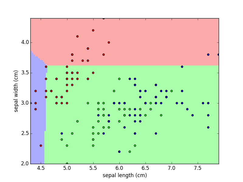
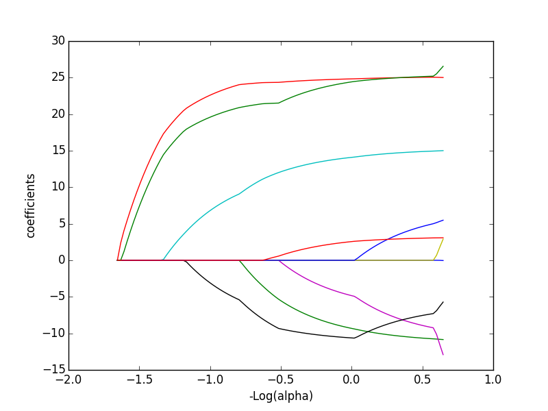
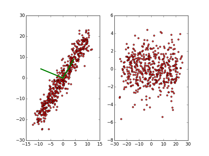
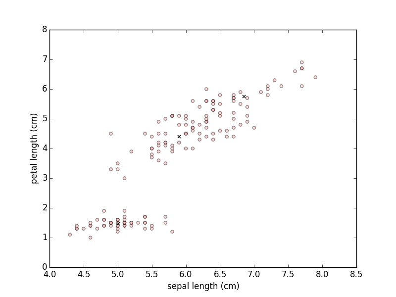
We'll cover, and you'll use, most or all of the following methods:
| Supervised | Unsupervised | |
|---|---|---|
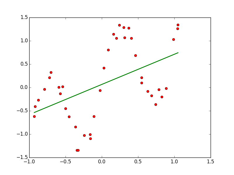
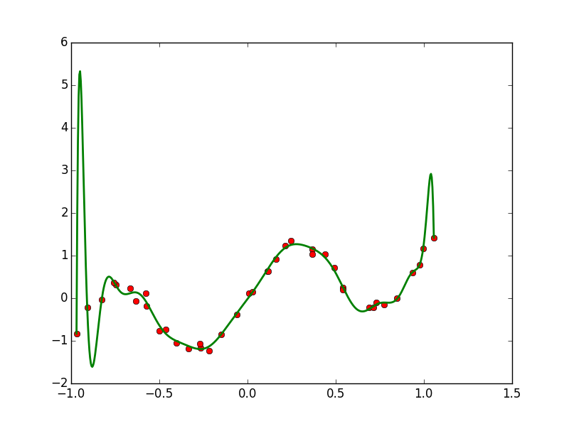
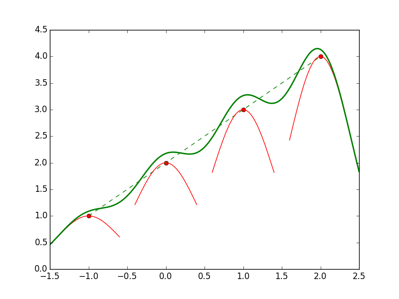
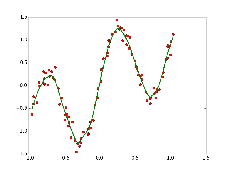
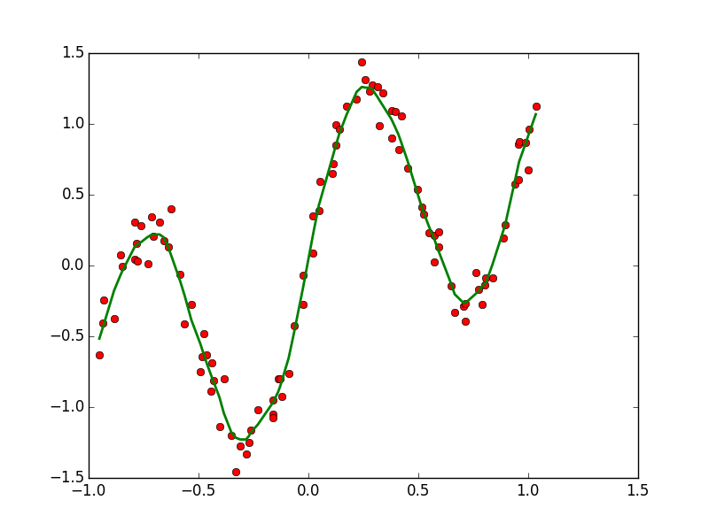
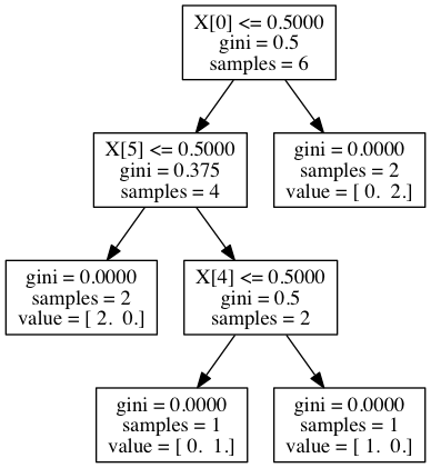
| CONTINUOUS | Regression: OLS, Lowess, Lasso | Variable Selection: PCA |
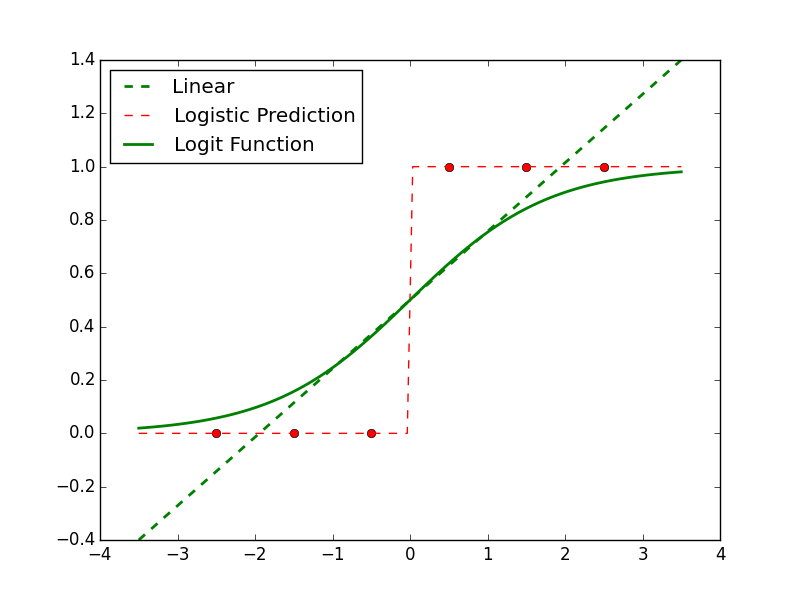
| DISCRETE | Classification: Logistic Regression, kNN, Decision Trees, Naive Bayes, Random Forest | Clustering: k-Means, Hierarchical Clustering |